The Strange Selection Bias in LASSO

Let’s suppose you have two variables \(X\) and \(Z\) that are positively correlated. \(X\) causes \(Y\) but \(Z\) does not.

n = 100
x <- rnorm(n)
z= x + rnorm(n)
x=scale(x)[,]
z=scale(z)[,]
y=x+rnorm(n)

The true value of \(\beta_z\) should be 0 and \(\beta_x\) should be 1 in the model \(y=\beta_x x + \beta_z z\). If we simulate this a bunch of times and estimate using OLS that’s exactly what we find on average. However, penalized regressions sacrifice the promise of unbiased estimates for other properties such as lower MSE and variable selection.

If we estimate the model using ridge regression, we end up seeing a substantial bias on \(\hat{\beta}_z\). The histogram below shows the distribution of ridge regression estimates of \(\beta_z\) from a ridge estimator with \(\lambda\) of 0.1.

simRidge <- function() {
  n = 100
  x <- rnorm(n)
  z= x + rnorm(n)
  x=scale(x)[,]
  z=scale(z)[,]
  y=x+rnorm(n)
  
  ridgemod<- lmridge(data = data.frame(y=y, x=x, z=z), 
          formula = y~x+z, K= 0.1)
  return(ridgemod$coef["z", ])
}

ridge.z.coefs <- replicate(1000, simRidge())
ggplot(data=  data.frame(Z = ridge.z.coefs), aes(x = Z)) + 
  geom_histogram() + geom_vline(xintercept = mean(ridge.z.coefs), 
                                colour = "red", linetype = 2)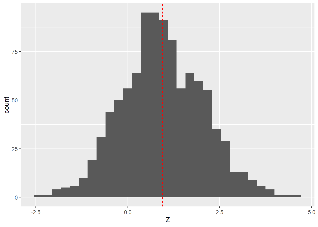

This is explicable when we examine the ridge regression loss function:

\[\begin{equation} L_{ridge}(\hat{\beta}_{ridge}) = \sum_{i=1}^{M}{ \bigg (y_i - \sum_{j=0}^{p} \hat{\beta}_{ridge_{j}} \cdot X[i, j] } \bigg ) ^2 + \frac{\lambda_2}{2} \sum^p_{j=1} {\hat{\beta}_{ridge_{j}}}^2 \end{equation}\]

The important part here is the squared penalty term. That means that the estimator will prefer adding mass to a smaller coefficient than a larger one. Suppose that \(\hat{\beta}_x\) is currently 1 \(\hat{\beta}_z\) is 0.1. That would create a ridge penalty of \(1^2+0.1^2=1.01\). If we add 0.1 to \(\hat{\beta}_x\), that increases the total ridge penalty to \(1.1^2+0.1^2=1.22\) whereas if we added 0.1 to \(\hat{\beta}_z\) it would only increase the ridge penalty to \(1^2+0.2^2=1.04\). That means the ridge loss function tends to find solutions where the parameter for a correlated variable gets some mass at the expense of the larger variable’s parameter. That is why we see \(\hat{\beta}_z\) get a positive value on average even though it is simulated as zero.

Where things get weird is when we do the same thing for LASSO. While the bias is much smaller than for ridge models, it’s still there and in the same direction.

simLasso <- function() {
  n = 100
  x <- rnorm(n)
  z= x + rnorm(n)
  x=scale(x)[,]
  z=scale(z)[,]
  y=x+rnorm(n)  
  
  
  gcdnetModel <- gcdnet(y = y,
                        x = cbind(x,z),
                        lambda = c(0.02), 
                        lambda2 = 0,
                        standardize = FALSE,
                        method = "ls")
  all.coefs <- coef(gcdnetModel)
  return(all.coefs["z", ])
}

lasso.z.coefs <- replicate(10000, simLasso())
ggplot(data=  data.frame(Z = lasso.z.coefs), aes(x = Z)) + 
  geom_histogram(bins = 100) + geom_vline(xintercept = mean(lasso.z.coefs), 
                                colour = "red", linetype = 2)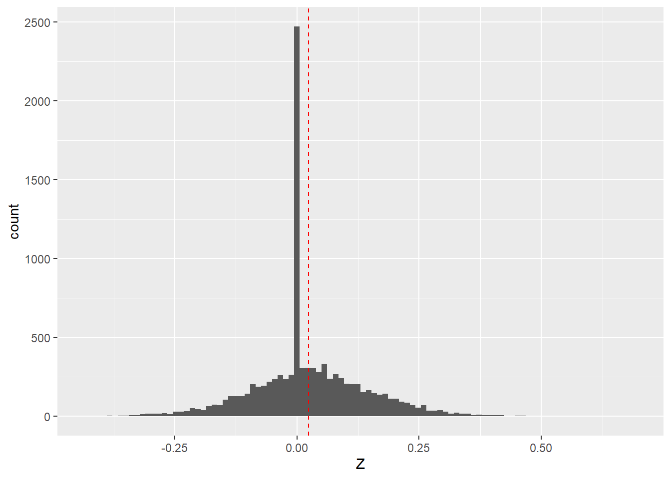

To see why that’s weird we can again consider the loss function:

\[\begin{equation} L_{lasso}(\hat{\beta}_{lasso}) = \sum_{i=1}^{M}{ \bigg (y_i - \sum_{j=0}^{p} \hat{\beta}_{lasso_{j}} \cdot X[i, j] } \bigg ) ^2 + \lambda_1 \sum^p_{j=1} {|\hat{\beta}_{lasso_{j}}|} \end{equation}\]

The important thing here is that the LASSO loss works on the absolute value of the coefficient. Taking our previous example, adding 0.1 to \(\hat{\beta}_x\), increases the total LASSO penalty to \(1.1+0.1=1.2\) exactly the same as if we added 0.1 to \(\hat{\beta}_z\) \(1+0.2=1.2\). In other words, the LASSO penalty should be indifferent between adding mass to \(\hat{\beta}_x\) and \(\hat{\beta}_z\). Given that we simulated \(\beta_z\) to be zero, it is odd that the LASSO estimate is positive on average.

I won’t detail all the dead ends we went down trying to figure this out, but I think we finally have the answer. The key is that while we simulate \(\beta_z\) to be zero, in each simulation, an OLS estimate puts some coefficient mass on \(\beta_z\). In the OLS estimates, this is symmetrically distributed around zero. Sometimes \(\beta_z\) is positive and sometimes negative. And it turns out that the LASSO estimator behaves quite differently depending on which of those scenarios is at play.

Estimating the model using LASSO generally decreases the magnitude of \(\hat{\beta}_x\). Lower values of \(\hat{\beta}_x\) increases the MSE of the model, which can potentially be reduced again by a larger magnitude of \(\hat{\beta}_z\). Of course, \(\hat{\beta}_z\) can also have a larger magnitude by modeling the same variance it did in the OLS estimate. It turns out that these two goals are overlapping when the OLS estimate of \(\beta_z\) was positive but work against each other when the OLS estimate of \(\beta_z\) was negative.

We capture where \(\hat{\beta}_z\) reduces the MSE by defining \(\epsilon_z\) as the residuals that \(\hat{\beta}_z\) changes in the OLS estimate. We calculate these by comparing the OLS predictions \(\hat{y}_{OLS}=\beta_{xOLS} x + \hat{\beta}_{zOLS} z\) to the predictions from the OLS model omitting the \(\hat{\beta}_{zOLS}\) term \(\hat{y}_{OLSnoZ}=\beta_{xOLS} x\). \(\epsilon_z= \hat{y}_{OLS} - \hat{y}_{OLSnoZ}\).

We then capture where reducing \(\hat{\beta}_x\) increased MSE by defining \(\epsilon_x\) as the residuals that are changed by reducing \(\hat{\beta}_x\) from its OLS value to its LASSO value. This time, we compare the OLS predictions to \(\hat{y}_{OLS}\) the OLS predictions if we swap \(\beta_{xOLS}\) for the LASSO value \(\beta_{xLASSO}\): \(\hat{y}_{lassox}=\beta_{xLASSO} x + \hat{\beta}_{zOLS} z\). That means we finally define \(\epsilon_x= \hat{y}_{OLS} - \hat{y}_{xLASSO}\).

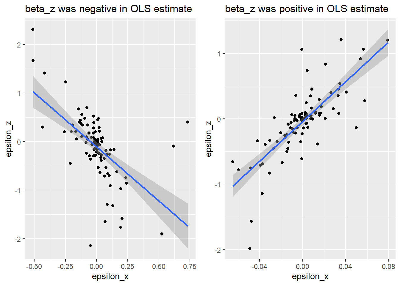
The following figure shows the relationship between the errors created by reducing \(\hat{\beta}_x\), \(\epsilon_x\), and the errors reduced in the OLS estimate by giving \(\hat{\beta_z}\) some coefficient mass: \(\epsilon_z\). For the case where \(\hat{\beta}_z\) was negative in the OLS estimate, the two goals come into conflict because there is a negative correlation between the observations that \(\hat{\beta}_z\) improves in the OLS estimate, and the variance that reducing \(\hat{\beta}_x\) opens up for modeling after it is penalized by LASSO. However, for a simulation where \(\hat{\beta}_z\) was positive in the OLS estimate, there is no tradeoff between these goals. A larger \(\hat{\beta}_z\) coefficient helps to mop up the variance that the penalization opened up and reduces prediction error for the observations it helped predict in the OLS estimate.

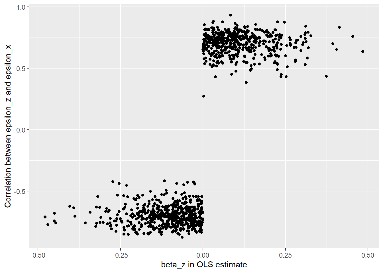
But those are just two simulations, does this pattern hold up more widely? The next figure shows the correlation between \(\epsilon_x\) and \(\epsilon_z\) for simulations where the OLS estimate of \(\beta_z\) took on different values. We see a sharp discontinuity at zero, where the correlation between the two types of variance available to model switches from positive to negative.

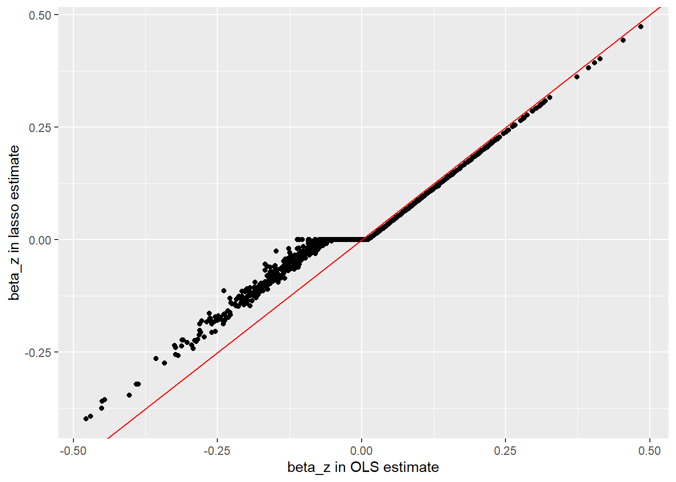
We can also plot the LASSO estimates for \(\beta_z\) against the OLS estimates. This shows a clear shift in behavior where \(\beta_z\) shifts from positive to negative in the OLS estimate.

Overall, this shows that penalized estimators can have some unexpected behavior because of the interaction between the least squares and penalty components of the loss function.